Session 1

Created Oct 2022, Last updated: 15 December, 2023

What is this page for?

This page has code for session 1 of BPI stats workshop. This session mainly focusses on R programming and is for beginners. We might not finish all of this in the session, but you will have the material for use later.

These exercises will only work if you have completed the pre-session items described here correctly. After following instructions on this page, go to the Session 2 page.

Create a new `Project`

Keep your work organised in RStudio by working within “Projects”. Start by creating a new project in a directory you want to save your work in.

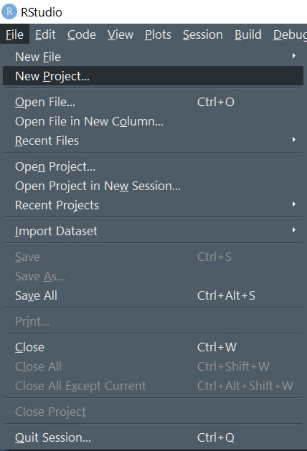
Create a new project by using File > New Project menu in RStudio.

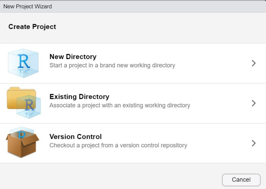
The new project dialogue box looks like this on Windows. Create a New Directory (e.g., Rstats_session1).

RMarkdown file

This is the best way to save analyses, including code and its output (e.g., graphs), along with formatted text. Outputs can be saved as Word, PDF or HTML files (HTML recommended).

A website like this one, which contains rich text, code and output, can be created entirely in RMarkdown format.

In RMarkdown files, writing *italics* converts text into italics, **bold** into bold and so on. This allows ‘rich text’ notes (e.g., to describe experiments and results).

R code is enclosed within ```{r}```

(three back ticks, curly bracket, small r followed by lines of code that ends with a new line of curly bracket and three back ticks). These are called code chunks.

Here are more examples from the RMarkdown cheatsheet.

Create your own RMarkdown result of this session

Knitting an R Markdown file

There will be an error if you have not installed all the packages required to knit an R Markdown file; first install the packages, then follow the code below.

To do this, create a new RMarkdown file by going to File -> New File -> R Markdown. This should open a new dialogue box in which you can name the new file as “Session1” and click OK.

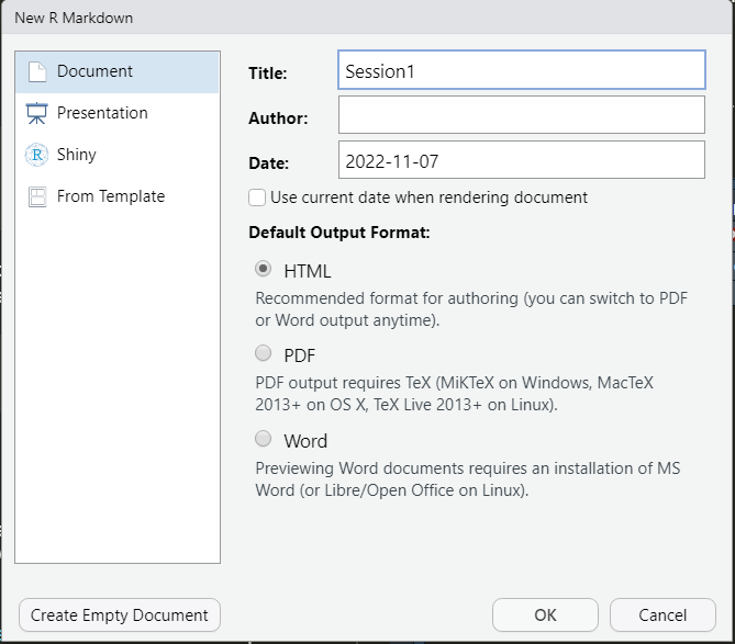
The new file is a generic template where the header with file details (title, output and date) is between three dashed lines --- at the top. This is called the YAML metadata or YAML header.

Text below this is code to be executed or just descriptive text. When the code and text is ready, use the Knit button on top of the pane to ‘knit’ the file into an HTML document (save it with a name such as “Session1.html”)

Create your RMarkdown file and write rest of today’s code within R chunks. This way you will have a record of the code and its output from this session.

The basic operators

Let’s look at the common operators in R.

1. assign operator <- (you can also use =). Pressing Alt and - together is the short-cut for this operator. You will use <- to assign values and create objects in R.

my_first_object <- "A"
my_second_object = "B"

2. common math operators are *, /, +, -, ^, and brackets ( )

5*2

[1] 10

2/10

[1] 0.2

3*20-10

[1] 50

3*(20-10)

[1] 30

2^2*5

[1] 20

2^(2*5)

[1] 1024

3. # at the start of line will indicate it is a comment and not something to be executed on the console. For example, typing 5*6 on the console will give you the result (30), but # 5*6 will not work because R thinks that’s a comment.

#multiplication 5*2

cars$speed * 20 #speeds multiplied by 20

 [1]  80  80 140 140 160 180 200 200 200 220 220 240 240 240 240 260 260 260 260
[20] 280 280 280 280 300 300 300 320 320 340 340 340 360 360 360 360 380 380 380
[39] 400 400 400 400 400 440 460 480 480 480 480 500

4. the square brackets [ ] have a special meaning, and typically used for sub-setting data frames (i.e., only picking rows in the table that match a criterion).

#pick the cell in row 2 and column 1
cars[2, 1]

[1] 4

#pick rows 2, 3, 4 and all columns 2
cars[c(2,3,4), 2]

[1] 10  4 22

#to pick all columns, leave blank after comma
cars[c(2,3,4), ]

  speed dist
2     4   10
3     7    4
4     7   22

#pick rows 1-10 in all columns
cars[1:10,]

   speed dist
1      4    2
2      4   10
3      7    4
4      7   22
5      8   16
6      9   10
7     10   18
8     10   26
9     10   34
10    11   17

5. the operator = is also used to assign an arugment of a function.

tail(cars, n = 10)

   speed dist
41    20   52
42    20   56
43    20   64
44    22   66
45    23   54
46    24   70
47    24   92
48    24   93
49    24  120
50    25   85

6. the $ operator is used to look up columns in a table.

cars$speed

 [1]  4  4  7  7  8  9 10 10 10 11 11 12 12 12 12 13 13 13 13 14 14 14 14 15 15
[26] 15 16 16 17 17 17 18 18 18 18 19 19 19 20 20 20 20 20 22 23 24 24 24 24 25

Operators can be combined.

cars$speed * 20

 [1]  80  80 140 140 160 180 200 200 200 220 220 240 240 240 240 260 260 260 260
[20] 280 280 280 280 300 300 300 320 320 340 340 340 360 360 360 360 380 380 380
[39] 400 400 400 400 400 440 460 480 480 480 480 500

#save the speed column as an object
car_speed <- cars$speed

7. logic operators such as == (equal to), != (not equal to), >= (equal to or greater than) or =< (equal to or less than). The object we saved above is called a vector. These are very common and we will come back to vectors later, but here’s how operators work on vectors.

#logical result in place for each item
car_speed > 20

 [1] FALSE FALSE FALSE FALSE FALSE FALSE FALSE FALSE FALSE FALSE FALSE FALSE
[13] FALSE FALSE FALSE FALSE FALSE FALSE FALSE FALSE FALSE FALSE FALSE FALSE
[25] FALSE FALSE FALSE FALSE FALSE FALSE FALSE FALSE FALSE FALSE FALSE FALSE
[37] FALSE FALSE FALSE FALSE FALSE FALSE FALSE  TRUE  TRUE  TRUE  TRUE  TRUE
[49]  TRUE  TRUE

car_speed == 4 | car_speed == 7 #vertical bar = or

 [1]  TRUE  TRUE  TRUE  TRUE FALSE FALSE FALSE FALSE FALSE FALSE FALSE FALSE
[13] FALSE FALSE FALSE FALSE FALSE FALSE FALSE FALSE FALSE FALSE FALSE FALSE
[25] FALSE FALSE FALSE FALSE FALSE FALSE FALSE FALSE FALSE FALSE FALSE FALSE
[37] FALSE FALSE FALSE FALSE FALSE FALSE FALSE FALSE FALSE FALSE FALSE FALSE
[49] FALSE FALSE

car_speed != 4

 [1] FALSE FALSE  TRUE  TRUE  TRUE  TRUE  TRUE  TRUE  TRUE  TRUE  TRUE  TRUE
[13]  TRUE  TRUE  TRUE  TRUE  TRUE  TRUE  TRUE  TRUE  TRUE  TRUE  TRUE  TRUE
[25]  TRUE  TRUE  TRUE  TRUE  TRUE  TRUE  TRUE  TRUE  TRUE  TRUE  TRUE  TRUE
[37]  TRUE  TRUE  TRUE  TRUE  TRUE  TRUE  TRUE  TRUE  TRUE  TRUE  TRUE  TRUE
[49]  TRUE  TRUE

#retrieve items from a vector with a [] brackets
car_speed[car_speed > 20]

[1] 22 23 24 24 24 24 25

car_speed[car_speed == 4]

[1] 4 4

Importing data from Excel

This is likely to be the most common thing we need to do before analysing data. This way we will also create our first object in R.

First, we will copy and save the two tables on the Data tables page, and then import those tables into RStudio.

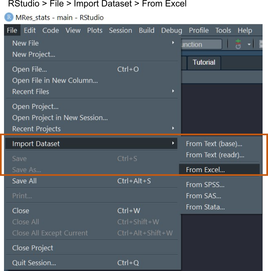
RStudio makes this easy through menu options, which only works if the package readxl is installed. In RStudio use the File > Import dataset > From Excel to import a sheet from an Excel file.

For this session, we will import a wide and long data table, which are saved in Sheet 1 and Sheet 2 of an Excel file called “Weights.xlsx”.

Excel file

You can download these “Mouse Weights” data as an Excel file from here.

Once you have the Excel file, import it into RStudio as follows. If all goes well, the code will appear on the console.

This is the code if data are imported ‘programmatically’ instead of the menu options in RStudio. Note the <- operator that assigns the output of the read_excel function with the argument path assigned using = to the name of the file we want to import given within double quote marks. We use the sheet argument to indicate which sheet to import (if we don’t, the default “Sheet 1” will be imported).

#start the package readxl
library(readxl)
#use the read_excel function
#name the imported table in Sheet1 as Weights 
Weights <- read_excel(path = "Weights.xlsx")
#name the imported table in Sheet2 as Weights_long
Weights_long <- read_excel("Weights.xlsx", 
                           sheet = "Sheet2")

These tables should appear as objects in the Environment pane of RStudio.

`data.frame` and its properties

Tables, also called data frames, are a very common type of object in R. This is an R object of class data.frame (examples of other classes are matrix and array). A tibble is a newer type of data.frame with some more features.

A vector is the most basic structure type in R, and it makes up other types of objects like data frames and lists.

`str`, `dim`, `head` and `$`

Common ways of checking the integrity and details of a data table are through these commands.

#structure of the Weights table
str(Weights)

tibble [10 × 3] (S3: tbl_df/tbl/data.frame)
 $ Mouse: chr [1:10] "A" "B" "C" "D" ...
 $ chow : num [1:10] 29.9 27.3 24 24.8 25.2 ...
 $ fat  : num [1:10] 28.3 29 29 24.6 34.6 ...

#structure of the Weights_long table
str(Weights_long)

tibble [20 × 3] (S3: tbl_df/tbl/data.frame)
 $ Diet      : chr [1:20] "chow" "chow" "chow" "chow" ...
 $ Bodyweight: num [1:20] 29.9 27.3 24 24.8 25.2 ...
 $ Mouse     : chr [1:20] "A" "B" "C" "D" ...

#dimensions of the table
dim(Weights)

[1] 10  3

#first 6 rows of the table
head(Weights)

# A tibble: 6 × 3
  Mouse  chow   fat
  <chr> <dbl> <dbl>
1 A      29.9  28.3
2 B      27.3  29.0
3 C      24.0  29.0
4 D      24.8  24.6
5 E      25.2  34.6
6 F      20.4  28.1

# the $ operator to access columns
Weights$Mouse

 [1] "A" "B" "C" "D" "E" "F" "G" "H" "I" "J"

Functions and arguments

Operations in R are carried out by calling various “functions”. Help on a function can be obtained by typing a ? and name of the function in the console.

Most functions will have arguments, or user-changeable settings that the function accepts. Several of them will have ‘default’ settings that will work in most scenarios. For example, the head function above by default shows 6 rows. This can be changed as necessary by using the argument n (for number of rows). n must always be an integer, otherwise there will be an error!

head(Weights, n = 2)

# A tibble: 2 × 3
  Mouse  chow   fat
  <chr> <dbl> <dbl>
1 A      29.9  28.3
2 B      27.3  29.0

Objects in R

We encountered tables (data.frame) above. Examples below include vectors and lists.

Vectors and lists

Other very common types of objects in R are a vector and list. A vector is a collection of items, but they have to be of the same type e.g., characters, numbers, logical operators (TRUE or FALSE), factors.

A list can be a collection of vectors or lists, and can therefore contain different types of items.

#a single character
variable1 <- "A"
#combine items into one variable vector with `c()`
#a character vector
vector1 <- c("A", "A", "B", "C", "C")
#check its type
class(vector1)

[1] "character"

#data.frame columns are a type of vectors
vector2 <- Weights$chow
#vector2 is numeric
class(vector2)

[1] "numeric"

#vector manipulation
vector2*2

 [1] 59.86 54.62 48.06 49.66 50.36 40.72 45.48 47.06 52.20 64.04

#coercing a vector type
vector3 <- as.character(vector2)
class(vector3)

[1] "character"

#create a list with list() function
list1 <- list(vector1, vector2)
list1

[[1]]
[1] "A" "A" "B" "C" "C"

[[2]]
 [1] 29.93 27.31 24.03 24.83 25.18 20.36 22.74 23.53 26.10 32.02

#see its class attribute
class(list1)

[1] "list"

Retrieving items from vectors

#item 2 from vector1
vector1[2]

[1] "A"

#subsetting a vector 
vector1[vector1 != "C"]

[1] "A" "A" "B"

#subsetting for items > 29 
vector2[vector2 > 29]

[1] 29.93 32.02

Subsetting vectors in-place

#logical operations on character vector
vector1 == "A"

[1]  TRUE  TRUE FALSE FALSE FALSE

#numeric logical operations on vector2
#items that match condition will return TRUE
vector2 > 29

 [1]  TRUE FALSE FALSE FALSE FALSE FALSE FALSE FALSE FALSE  TRUE

Subsetting data frames

For data frames, a comma separates subsetting of rows and columns in the data.frame[row, column] indexing format.

To select rows based on a condition, first select the name of the column to set the condition with $. If this part is left blank, all rows are selected.

#rows where chow > 25
Weights[Weights$chow > 25,]

# A tibble: 5 × 3
  Mouse  chow   fat
  <chr> <dbl> <dbl>
1 A      29.9  28.3
2 B      27.3  29.0
3 E      25.2  34.6
4 I      26.1  27.7
5 J      32.0  35.0

#rows where chow > 25 and column fat in output
Weights[Weights$chow > 25, "fat"]

# A tibble: 5 × 1
    fat
  <dbl>
1  28.3
2  29.0
3  34.6
4  27.7
5  35.0

#with a vector of column names
Weights[Weights$chow > 25, c("Mouse", "fat")]

# A tibble: 5 × 2
  Mouse   fat
  <chr> <dbl>
1 A      28.3
2 B      29.0
3 E      34.6
4 I      27.7
5 J      35.0

#all rows in column Mouse
Weights[, "Mouse"]

# A tibble: 10 × 1
   Mouse
   <chr>
 1 A    
 2 B    
 3 C    
 4 D    
 5 E    
 6 F    
 7 G    
 8 H    
 9 I    
10 J

Subsetting and retrieving items from lists

This is similar to handling vectors, but you may need to use [[ double brackets to first select the item in the list.

#retrieving item 3 from list 1 in list1
#note the double [ (`[[`)
list1[[1]][3]

[1] "B"

#retrieve item and operate on it
list1[[2]][3]*2

[1] 48.06

#subsetting a list
#[[ ]]to get the sub-vector, then subsetting with []
list1[[1]][list1[[1]] != "A"]

[1] "B" "C" "C"

#logical operations on lists 
list1[[1]] == "A"

[1]  TRUE  TRUE FALSE FALSE FALSE

Plotting a graph

Using the package `grafify`

For simplicity we will use grafify instead of ggplot2. The grafify package provides a set of functions that calls ggplot2 to plot graphs with fewer lines of code. This is handy for repeatedly plotting graphs while exploring data.

grafify

There will be an error if you have not installed grafify and/or its dependencies, first install the packages, then follow the code below.

#start the grafify package
library(grafify)

Loading required package: ggplot2

#box and whisker plot
plot_scatterbox(data = Weights_long, 
                xcol = Diet,
                ycol = Bodyweight)

#lots of further optimisations are possible
#see https://grafify-vignettes.netlify.app

Using the package `ggplot2`

This is a simple code to produce a box and whiskers plot; lots and lots of tweaks are possible and almost every little thing can be changed from ‘default’.

ggplot(data = Weights_long, 
       aes(x = Diet, y = Bodyweight))+
  geom_boxplot(aes(fill = Diet))+
  geom_jitter()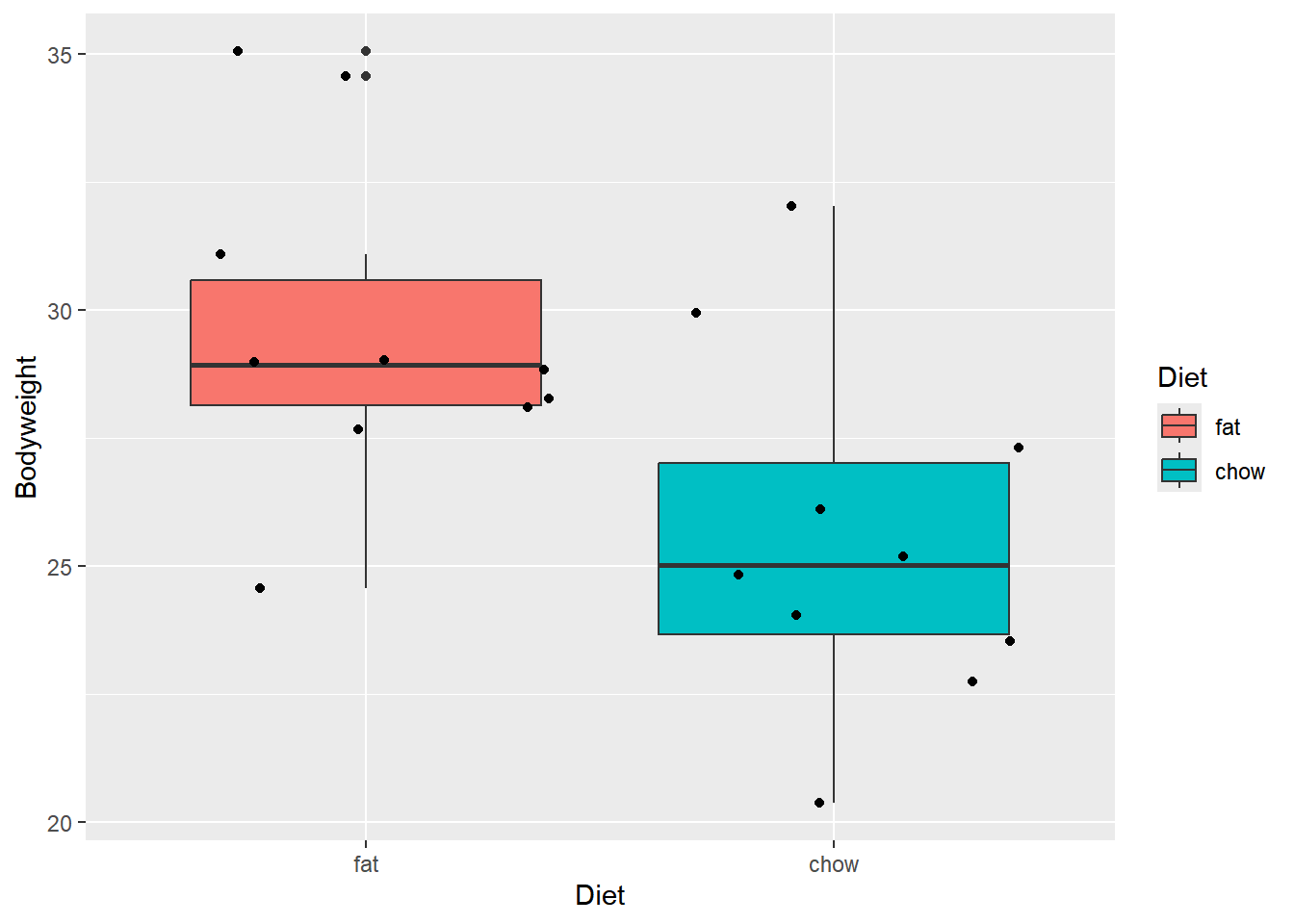

Student’s t test

Formula input with long table

Let’s perform a simple t test in R. The standard ‘formula’ notation is Y ~ X for data in long format. This is read as Y is predicted by X. Y is the dependent variable (Bodyweight in this case), which is predicted by the independent variable, or categorical factor, X (Diet in this case).

The symbol ~ (tilde) has special meaning in R and is used in formulas as above to separate the dependent and independent variables.

t.test(Bodyweight ~ Diet,
       data = Weights_long)


    Welch Two Sample t-test

data:  Bodyweight by Diet
t = -2.7058, df = 17.892, p-value = 0.01453
alternative hypothesis: true difference in means between group chow and group fat is not equal to 0
95 percent confidence interval:
 -7.1178367 -0.8941633
sample estimates:
mean in group chow  mean in group fat 
            25.603             29.609

Column names with wide table

If data are in wide format, the same t.test function can be used with first two arguments as the two columns to be tested. Note that the results are the same.

t.test(Weights$chow, Weights$fat)


    Welch Two Sample t-test

data:  Weights$chow and Weights$fat
t = -2.7058, df = 17.892, p-value = 0.01453
alternative hypothesis: true difference in means is not equal to 0
95 percent confidence interval:
 -7.1178367 -0.8941633
sample estimates:
mean of x mean of y 
   25.603    29.609

Columns as factors for t-tests and ANOVAs

Student’s t test (when comparing exactly 2 groups) and ANOVAs (analysis of variance; used when there are more than 2 groups being compared) require groups as discreet or categorical variables (e.g., Untreated & Treated, WT vs KO, Boys vs Girls). In R, such categorical variables should be encoded in data frames as “factors”. Columns with such data should be converted to factor data type using the as.factor function.

In the long data table, we have one factor (Diet) with two levels (“chow” and “fat”), and various observations of Bodyweight fall within these two levels. Mouse is also a factor with 10 levels (A-J).

Weights_long$Diet <- as.factor(Weights_long$Diet)
Weights_long$Mouse <- as.factor(Weights_long$Mouse)
#check the structure
str(Weights_long) #compare with previous result above

tibble [20 × 3] (S3: tbl_df/tbl/data.frame)
 $ Diet      : Factor w/ 2 levels "chow","fat": 1 1 1 1 1 1 1 1 1 1 ...
 $ Bodyweight: num [1:20] 29.9 27.3 24 24.8 25.2 ...
 $ Mouse     : Factor w/ 10 levels "A","B","C","D",..: 1 2 3 4 5 6 7 8 9 10 ...

#check levels in a factor
levels(Weights_long$Diet) #"chow" and "fat"

[1] "chow" "fat"

#number of levels
nlevels(Weights_long$Diet)

[1] 2

#numeric vector converted into factor
vector3 <- as.factor(vector2)
str(vector3)

 Factor w/ 10 levels "20.36","22.74",..: 9 8 4 5 6 1 2 3 7 10

#numeric operation will now fail
vector3*2

Warning in Ops.factor(vector3, 2): '*' not meaningful for factors

 [1] NA NA NA NA NA NA NA NA NA NA

By default, R will order factors alphabetically or ascending if numbers. This order will also be followed for graphs, but can be changed if required.

#change order of levels as "fat" & "chow"
Weights_long$Diet <- factor(Weights_long$Diet, #select column Diet
                            levels = c("fat", "chow")) #vector in desired order

#plot and compare with output above
plot_scatterbox(data = Weights_long, 
                xcol = Diet,
                ycol = Bodyweight)

factor and as.factor are somewhat “advanced” functions while beginning R, but they are required to perform ANOVAs correctly!

Categorical variables as factors

It is advisable to get into the habit of converting columns with categorical variables into factors immediately after importing the data frame into R. This is important for calculating ANOVAs correctly.

Read more about factors in the R for Data Science book and on this link to software carpentry.

Table summaries

There are many ways of getting summaries such as mean and SD for variables in a table. The most common way is to use the tidyverse way. In addition, grafify as a simple function that provides summaries based on groups.

Tidyverse method with `dplyr`

#start the dplyr package
library(dplyr)

Warning: package 'dplyr' was built under R version 4.3.2


Attaching package: 'dplyr'

The following objects are masked from 'package:stats':

    filter, lag

The following objects are masked from 'package:base':

    intersect, setdiff, setequal, union

Weights_long %>%         #%>% is called the pipe
  group_by(Diet) %>%     #variable to group by
  summarise(Mean = mean(Bodyweight),   #mean
            SD = sd(Bodyweight),       #SD 
            Median = median(Bodyweight), #Median
            Count = length(Bodyweight))  #Count

# A tibble: 2 × 5
  Diet   Mean    SD Median Count
  <fct> <dbl> <dbl>  <dbl> <int>
1 fat    29.6  3.18   28.9    10
2 chow   25.6  3.44   25.0    10

`grafify` method

There is simple function called table_summary in grafify to do this.

table_summary(data = Weights_long, #table name
              Ycol = "Bodyweight", #numeric variable
              ByGroup = "Diet")   #grouping variable(s)

  Diet Bodyweight.Mean Bodyweight.Median Bodyweight.SD Bodyweight.Count
1  fat          29.609            28.915      3.179509               10
2 chow          25.603            25.005      3.436659               10

Today’s code for Rmarkdown

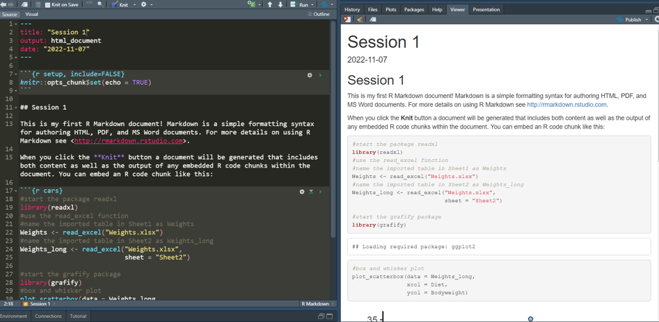
Copy all following lines of code inside an R code chunks in the .rmd file. You can add plain or rich text as you like outside the code to describe the code!

#start the package readxl
library(readxl)
#use the read_excel function
#name the imported table in Sheet1 as Weights 
Weights <- read_excel("Weights.xlsx")
#name the imported table in Sheet2 as Weights_long
Weights_long <- read_excel("Weights.xlsx", 
                           sheet = "Sheet2")

#start the grafify package
library(grafify)
#box and whisker plot
plot_scatterbox(data = Weights_long, 
                xcol = Diet,
                ycol = Bodyweight)

#perform a t.test
t.test(Bodyweight ~ Diet,
       data = Weights_long)

If all goes OK, you should see the ‘output’ and code in the new R Markdown file in the Viewer pane. The R Markdown and HTML files are your record of the code used for the analyses and its output (along with the raw data in the Excel file).

RMarkdown is ‘blind’ to the current environment

R Markdown files will only work if all objects required for the code are created and/or imported within that file. It will not “look for” objects in your Environment - objects have to be created by the code within the R Markdown. This is by design. It is a good feature because if you share your R Markdown file with colleagues, it will still work!

Similarly, ‘kitting’ an R Markdown file does not create any new objects in your Environment.

In the examples from session 1, the “Weights” data frame needs to be imported and created within the R Markdown document even though you might already have it in your Environment. Without the lines of code that import the data, the rest of the code will not work!

Happy R’ing!

What is this page for?

Create a new Project

RMarkdown file

Create your own RMarkdown result of this session

The basic operators

Importing data from Excel

Excel file

data.frame and its properties

str, dim, head and $

Functions and arguments

Objects in R

Vectors and lists

Retrieving items from vectors

Subsetting vectors in-place

Subsetting data frames

Subsetting and retrieving items from lists

Plotting a graph

Using the package grafify

Using the package ggplot2

Student’s t test

Formula input with long table

Column names with wide table

Columns as factors for t-tests and ANOVAs

Table summaries

Tidyverse method with dplyr

grafify method

Today’s code for Rmarkdown

Create a new `Project`

`data.frame` and its properties

`str`, `dim`, `head` and `$`

Using the package `grafify`

Using the package `ggplot2`

Tidyverse method with `dplyr`

`grafify` method