Pre-session 1 instructions
What is this page for?
This page has instructions for installing R & RStudio on your laptops and confirming they are working all right. This is to ensure that we are ready for Stats Workshop session 1. This activity will likely take around 30 min to complete.
After following instructions on this page, go to Session 1 and Session 2 pages.
R/Studio & package versions
Even if you have previously installed R/RStudio or ggplot2 or other packages, please re-install the latest versions. Old versions are likely to lead to errors during the workshops.
Get latest versions even if you have used R before
If you have previous versions or R and/or RStudio, please uninstall them and re-install their latest versions as below.
We will use the latest R and RStudio, and various packages, therefore please read this page to ensure we all have working copies of required software.
Installation steps
Follow the steps in this order.
R is freely available from The Comprehensive R Archive Network (CRAN). Go to the CRAN website and use the links at the top for your OS (operating system, e.g., Windows or MacOS or Linux) to download and install R. Use default options during installation.
RStudio Desktop is a free IDE (integrated development environment) that makes it very easy to use R that we installed in step 1. Go to the RStudio website and install their free RStudio Desktop version for your OS. Use default options during installation. Note that RStudio was recently renamed “Posit”, but nothing has changed for users. I still call it RStudio.
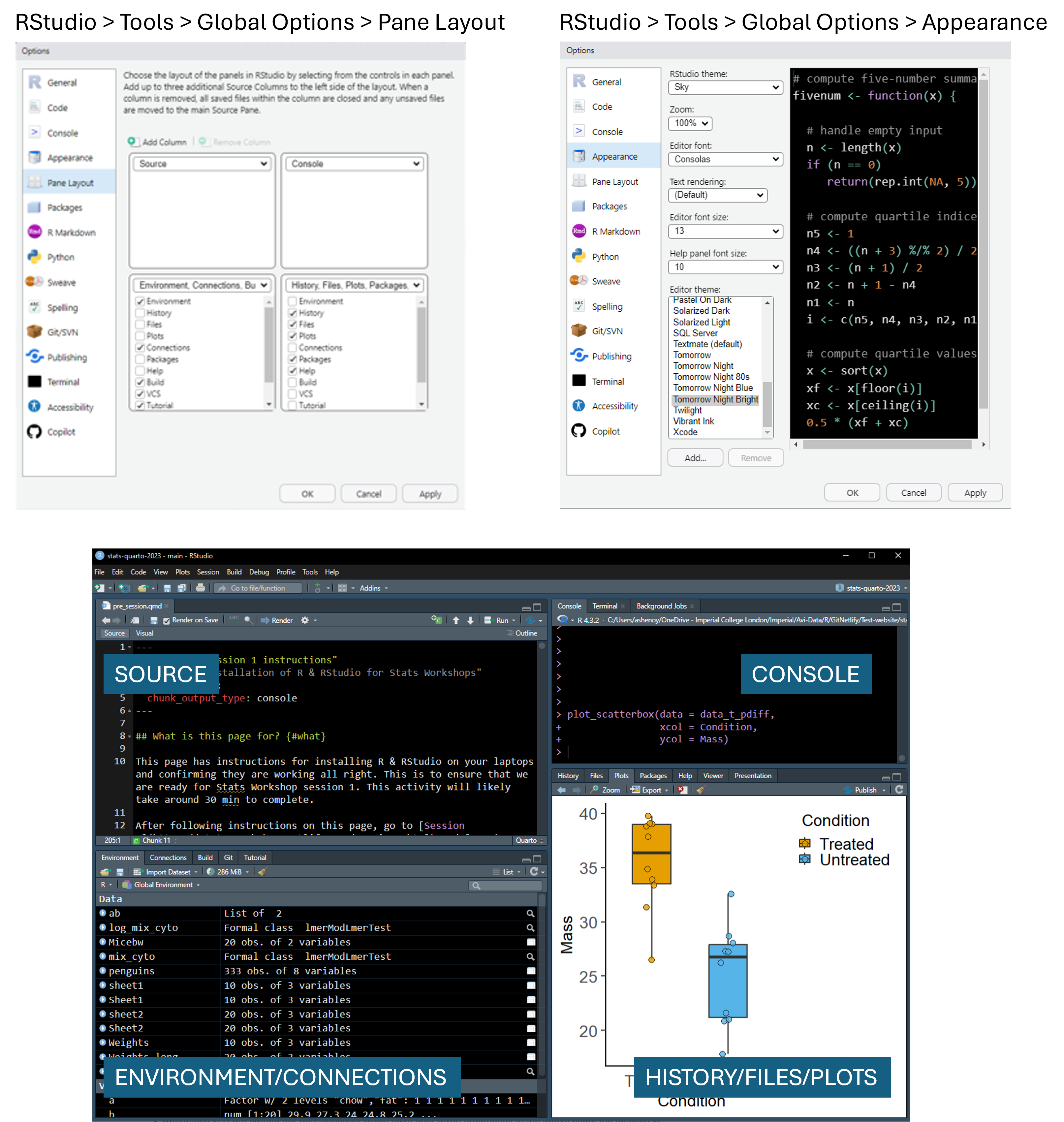
Open RStudio and familiarise yourself with the four windows or “panes”. You could start by watching these short videos (will likely need Imperial login to access the Sharepoint site), the first one Getting started with R - intro session 1 explains the installation process.
The pane you need for next steps is the ‘Console’. It’ll have a blinking cursor.
My RStudio looks like this image below. I changed the default pane layout by going to the dialogue boxes as below. I prefer a dark background, but you can use settings you prefer!
- For the workshop, we will need several graphing and statistics packages. To install them, copy the code below to your ‘Console’ and hit ENTER to run it. You can use the
Copyicon at the top right of the code chunks below.
It could take several minutes to download and install all required packages. Note that R is case sensitive (knitr is not the same as Knitr, KNITR or other variants).
install.packages(pkgs = c("rmarkdown",
                          "knitr",
                          "readr",
                          "readxl",
                          "grafify",
                          "pwr",
                          "effectsize",
                          "palmerpenguins"),
                 dependencies = TRUE)
The above code will download and install packages called rmarkdown & knitr (for creating and saving code and graphs), readr & readxl (for reading data from Excel files), grafify (for graphs and ANOVA), pwr and effectsize for power calculations, and palmerpenguins (a dataset of measurements taken at the Palmer Station, Antarctica), and any packages that they depend on. This can take some time depending on download speeds etc.
Functions and their arguments
Operations in R are carried out with functions, which have user-given arguments. In the code above, the function we use is install.packages(). We have also set two arguments, pkgs and dependencies. The values we set instruct the function to do what we want it to.
Depending on your OS and other settings, during the installation process you might be asked questions, for example:

For this question, it is good to say “Yes” once; if it asks the same again, say “No” and proceed.
Another question could be:
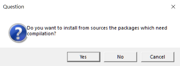
Say “No” and proceed (building from source needs more software and can be much more time-consuming).
What if there are errors?
The easiest thing to do if there are errors is to copy the text of the error and do a Google search. Almost all errors have been experienced by other users and there may be help online to resolve them.
The basic operators
Let’s look at the common operators in R. You can copy the code below to your console to familiarise yourself with basic operations.
- assign operator
<-(you can also use=). PressingAltand-together is the short-cut for this operator. You will use<-to assign values and create objects in R. The<-can also be used to generate and save new columns in a data table (see step 6 below).
Create your first objects as below. Alpha and five will appear in your Environment pane.
#an object with an alphabet
Alpha <- "A"
#an object with one number
five <- 5- hash
#at the start of line will indicate it is a comment and not something to be executed on the console. For example, typing5*6on the console will give you the result (30), but# 5*6will not work because R thinks that’s a comment.
Comments can be added at the end of a line of code. This is very useful to do and highly recommended. You should explain what your line of code is doing so that when you read your code a year later, you are reminded of the rationale behind those steps. Or when you share your code with someone else, they’ll understand the steps of your analysis.
- arithmetic operators that are common:
*,/,+,-,^, and brackets(). Priority of processing is BODMAS (Brackets, Order of power or roots, Division/Multiplication, Addition/Subtraction).
# a comment
7 * 3 #three times seven
[1] 21#7 * 3 is also a comment
#mathematical operation on an object
five * 5 [1] 25#this will fail with an error message
Alpha * 5dollar
$operator is used to look up columns in a table. The double square brackets[[ ]]do similar things and has special meaning in R.the equal operator
=is also used to assign anarugmentof afunction.
cars is a table in base R, let’s use it as an example. head is a function to see the rows from the start of a table. Let’s use this function on the table cars.
head(cars) #shows top 6 rows by default speed dist
1 4 2
2 4 10
3 7 4
4 7 22
5 8 16
6 9 10#with a value to an argument for head
head(cars, n = 3) #show first 3 rows speed dist
1 4 2
2 4 10
3 7 4#see the table cars
View(cars)
#pick the column speed from cars
cars$speed [1] 4 4 7 7 8 9 10 10 10 11 11 12 12 12 12 13 13 13 13 14 14 14 14 15 15
[26] 15 16 16 17 17 17 18 18 18 18 19 19 19 20 20 20 20 20 22 23 24 24 24 24 25#same as above with double square brackets
cars[["speed"]] [1] 4 4 7 7 8 9 10 10 10 11 11 12 12 12 12 13 13 13 13 14 14 14 14 15 15
[26] 15 16 16 17 17 17 18 18 18 18 19 19 19 20 20 20 20 20 22 23 24 24 24 24 25#mathematical operation on the column
cars$speed + 10 [1] 14 14 17 17 18 19 20 20 20 21 21 22 22 22 22 23 23 23 23 24 24 24 24 25 25
[26] 25 26 26 27 27 27 28 28 28 28 29 29 29 30 30 30 30 30 32 33 34 34 34 34 35Other operators we will look at in Session 1 are:
the single square brackets
[]have a special meaning, and typically used for sub-setting data frames (i.e., only picking rows in the table that match a criterion).logic or boolean operators such as
==(equal to),!=(not equal to),>=(equal to or greater than) or=<(equal to or less than).TRUEandFALSEare special terms (always capitals), and cannot be used as variable names.quotation marks in pairs are common: both
'and"are the same, use what you prefer. The backward tick ` has special uses and is not the same as single or double apostrophes. Names of columns passed to[[ ]]need to be in quotation marks. The name of an object stored in the Environment is used without quotation marks (note that we didn’t use quotation marks aroundfivewhen we usedfive * 5above).
Variables
Variables are named objects saved to the Environment (not written to a folder yet). In point 1 above we created variables Alpha and five. Variables should have unique names, otherwise they will be written over. Use short, sensible names that do not start with a number. Variables can contain various data types.
Check installation
Check that everything has gone OK by loading one of the packages we installed, and using it to plot a graph.
This leads us to another important aspect of using R. To save memory, R does not “load” all available packages - the user must invoke them explicitly by using the library function. Once a package is loaded, all of its features are available for use.
Checking the installation is therefore a two-step process.
- First copy the following line to your console and hit ENTER (this will make the
grafifypackage available to use). It will only work if your installation of the packagegrafifywent OK!
#invoke the grafify package
library(grafify)- Second, copy the line below to your console and hit ENTER. It should produce a graph using the
grafifypackage.
#use the plot_scatterbox function from grafify
plot_scatterbox(data_t_pdiff, Condition, Mass)
If all went OK, a graph with scattered symbols with box and whiskers should appear in the Plots pane.

In the function above, we used a data table from the grafify package and used the function plot_scatterbox. First, let’s look at the data table, or more commonly called a data frame in R.
#View function opens the table in the source pane
View(data_t_pdiff)

#names of columns
names(data_t_pdiff)
[1] "Subject" "Condition" "Mass" #structure of the table
str(data_t_pdiff)'data.frame': 20 obs. of 3 variables:
$ Subject : Factor w/ 10 levels "A","B","C","D",..: 1 1 2 2 3 3 4 4 5 5 ...
$ Condition: Factor w/ 2 levels "Treated","Untreated": 2 1 2 1 2 1 2 1 2 1 ...
$ Mass : num 20.9 33.4 21 33.9 28.7 ...You now see that the table has 3 columns, Subject (an ID of each mouse used in the study), Condition (whether a mouse was Treated or Untreated with a drug) and Mass (its body weight in grams).
When we plotted the graph above, we used the first three arguments in their default order. We can be more explicit as below.
plot_scatterbox(data = data_t_pdiff,    #name of data frame
                xcol = Condition,       #column to plot on X axis
                ycol = Mass)            #column to plot on Y axis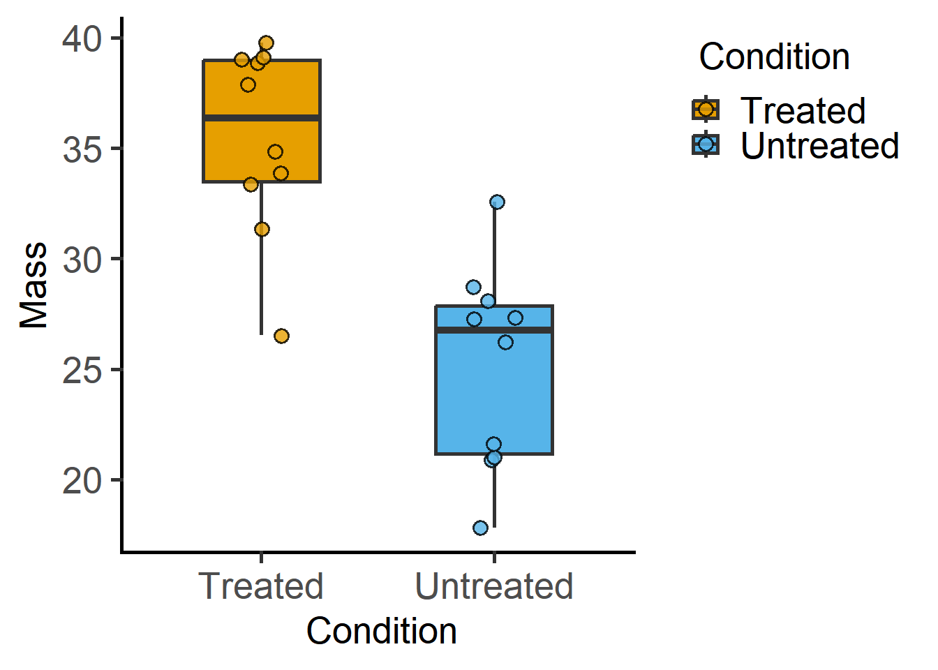
No one can remember the arguments, let alone their order for all the functions in R. But do not worry, help is nearby. Adding a ? before the name of the function gives you usage details in the Help pane.
?plot_scatterbox()This is how help looks on my Rstudio. As you can see, there are many arguments to tweak the graph, most of which have sensible defaults. We will rarely need to assign a value to all of them, but it’s good to know what can be changed in this graph.
If you are interested in tweaking this graph further, the grafify vignettes website has detailed examples.

Further exercises
Go to Session 1 if you’d like to try out more things in R!
Additional resources
Additional helpful resources listed here at the Statistics for Micro/Immuno-biologists website.